Multivariate Analysis and Metabolite ID-ing

Multivariate Statistical Analysis

This tutorial illustrates a multivariate statistical analysis workflow for NMR-based metabolic profiling using the metabom8 R package.

Example Data

Proton (¹H) NMR data are available in the nmrdata package (www.github.com/tkimhofer/nmrData) and constitute standard 1D experiments acquired from murine urine samples. Information on experimental setup and NMR data acquisition can be found in the original publication¹.

library(metabom8)

Here, pre-processed data are imported.

# Load data
data(bariatric)

# Declare variables
Xn<-bariatric$X.pqn # PQN-normalised NMR data matrix
dim(Xn)
#> [1]    67 56357

ppm<-bariatric$ppm     # chemical shift vector in ppm
length(ppm)
#> [1] 56357

meta<-bariatric$meta   # spectrometer metadata
dim(meta)
#> [1]  67 417

an<-bariatric$an       # sample annotation
dim(an)
#> [1] 67  4

The following variables should be in the R workspace after executing the code snippet above:

Xn - preprocessed NMR data matrix where rows represent spectra and columns represent ppm variables
ppm - chemical shift vector in part per million (ppm), it’s length equals to the number of columns of Xn length(ppm)==ncol(Xn)
an - sample annotation data frame containing information about each sample (e.g. group membership, confounder variables)
meta - spectrometer metadata, e.g., probe temperature at acquisition (not essential for this tutorial)

Interactive visualisation of NMR spectra

The following plotly-based functions are available to visualise and browse NMR spectra interactively:

spec(Xn[1,], ppm, shift = c(0,10)) # singe spectrum, interactive

matspec(Xn[1:10,], ppm, shift = c(0.8, 1))  # spectral overlay, interactive

PCA - Unsupervised Analysis

In metabom8, Principal Component Analysis (PCA) can be performed using the pca() function. This function takes the NMR matrix (X = Xn), the desired number of principal components (pc = 2), and optional centering and scaling parameters (e.g., center = TRUE, scale = “UV” for unit variance scaling).

# Perform PCA
pca_model=pca(X=Xn, pc=2, scale='UV', center=TRUE)

The returned object, pca_model, is a structured S3 object containing model information such as:

t – scores matrix (projections of samples onto each PC)
p – loadings matrix (variable contributions to each PC)
$R^2X$ – explained variance per component
other internal diagnostics

Why use `metabom8::pca()`?

Unlike generic PCA functions (e.g., prcomp()), metabom8::pca() returns an object fully compatible with the rest of the metabom8 ecosystem. This allows:

Streamlined model visualisation using helper functions like plotscores() and plotload()
Consistent aesthetics and annotations (e.g., point grouping, labelling)
Reusability of the PCA object for further interpretation and diagnostics
Simplified code flow for multivariate chemometric pipelines

Visualising PCA Results

The pca() function in metabom8 returns a structured PCA model, directly compatible with downstream visualisation functions. Use plotscores() for scores plots and plotload() for loadings.

Each point in the scores plot represents a sample in Principal Component (PC) space. Axis labels show explained variance ( $R^2$ ), and the dotted ellipse denotes Hotelling’s $T^2$ for outlier detection.

Aesthetic mapping (colour, shape, labels) is flexible via the an list:

# define scores that should be labelled
idx<-which(pca_model@t[,1]>200 | pca_model@t[,2]>200 & an$Class=='RYGB') # PC 2 scores above 20 and in group RYGB

# construct label vector with mouse IDs
outliers <- rep("", nrow(an)); outliers[idx] <- an$ID[idx]

# Plot PCA scores, colour according to class, point shape according to time of sample collection and label outliers
plotscores(
  obj=pca_model, 
  pc=c(1,2), 
  an=list(
    Class=an$Class,         # point colour
    Timepoint=an$Timepoint, # point shape
    ID=outliers             # point label
  ),  
  title='PCA - Scores plot')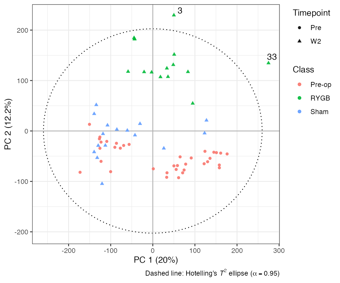

Loadings are visualised as line plots resembling NMR spectra. These are either backscaled (loading value multiplied by spectral variable’s standard deviation) or statistically reconstructed (cor/cov of PC score and spectral variable). Resulting loadings plot reveals variable contributions to each PC:

# Focused loadings plot of PC 2 (aromatic region)
plotload(pca_model, pc = 2, shift = c(6, 9), type='backscaled')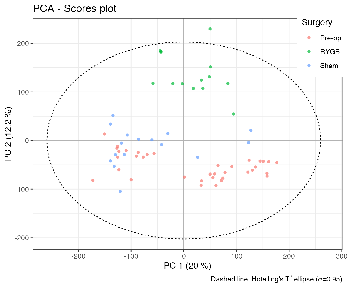

The x-axis shows chemical shift (ppm); the y-axis reflects loading magnitude; colour indicates normalised importance. Loadings and scores are linked—peaks with warm colours correspond to sample trends in the scores plot.

# Focused loadings plot of PC 2 (aromatic region)
specload(pca_model, 
         pc = 2, 
         shift = c(7.4, 7.6),
         an=list(
            facet=pca_model@t[,2]>0, 
            type='backscaled', 
            alp = 0.5, 
            title = 'Overlayed Spectra with Backscaled Loadings'
         )
)

Supervised Analysis with O-PLS

While PCA revealed clustering by treatment group, it does not explicitly model group differences. To directly associate spectral variation with an outcome, we use Orthogonal Partial Least Squares (O-PLS), implemented via opls() in metabom8.

O-PLS decomposes the NMR matrix $X$ into:

a predictive component aligned with the outcome variable $Y$
one or more orthogonal components capturing structured variation unrelated to $Y$

This separation improves model interpretability and helps isolate biologically meaningful variation.

Model Training

# Exclude pre-op group
idx<-an$Class!='Pre-op'
X<-Xn[idx,]
Y<-an$Class[idx]

# Train O-PLS model
opls.model<-opls(X,Y)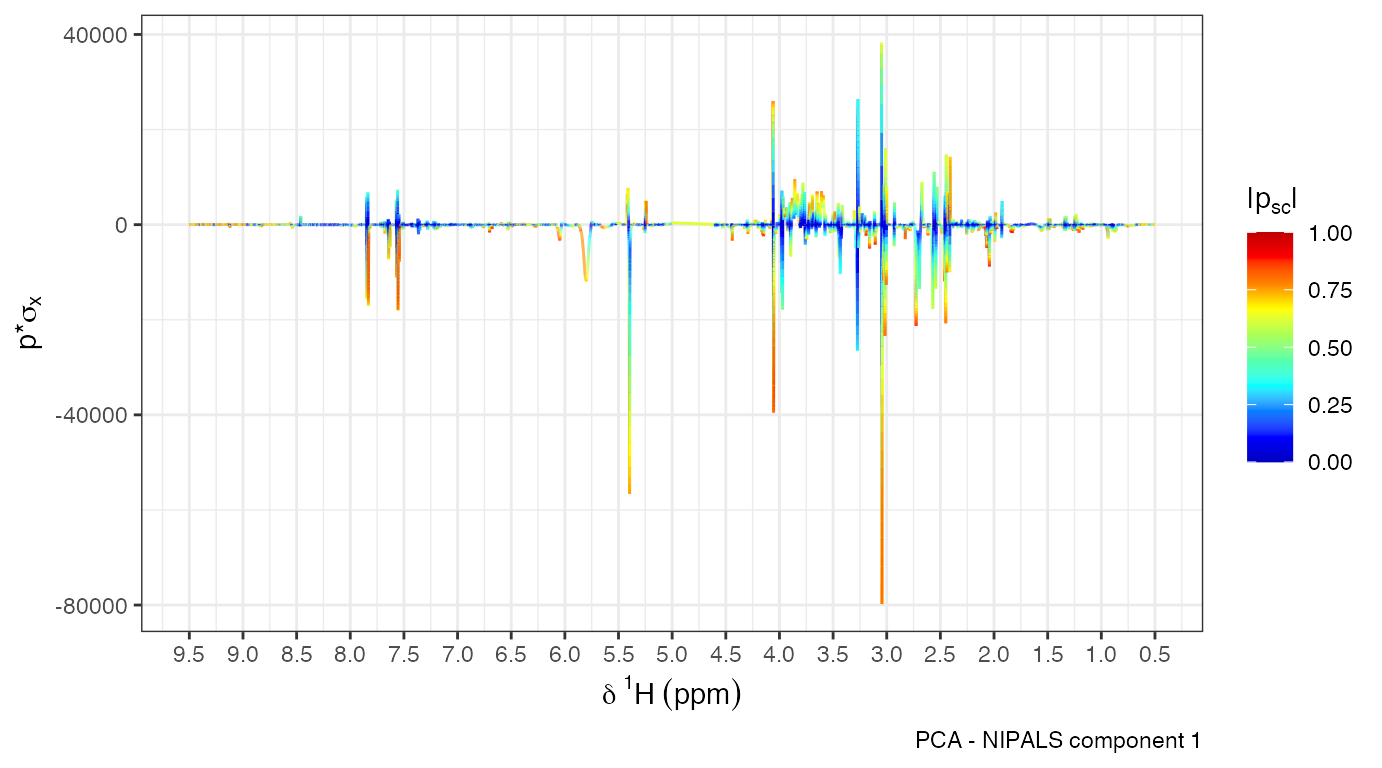

The model summary plot displays configurations tested (e.g., 1+1 predictive+orthogonal components). The selected model minimizes overfitting using internal cross-validation.

summary(opls.model)

$R^2X$ : proportion of variance explained in the predictor matrix (X)
$R^2Y$ : proportion of variance explained in the outcome variable (Y)
$Q^2$ / $AUROC_{CV}$ : cross-validated prediction accuracy

Overfitting & Component Selection

To guide model complexity, metabom8 automatically determines the optimal number of orthogonal components using internal cross-validation. The algorithm incrementally adds orthogonal components and evaluates the improvement in predictive performance. For continuous outcomes, selection is based on changes in $Q^2$ ; for classification problems, the increase in cross-validated AUROC ( $\Delta$ AUROC $_{CV}$ ) is monitored. A new component is retained only if it improves performance beyond a minimum threshold ( $\Delta > 0.05$ ), helping to avoid overfitting on noise or technical variance.

How many orthogonal components should I fit?

To further support model validation, permutation testing can be applied via the opls_perm() function. This procedure assesses whether the model’s performance could arise by chance, by randomly permuting Y labels and re-fitting the model multiple times. When deciding whether to retain an additional component, comparing the observed improvement (e.g., in AUROC or $Q^2$ ) against the distribution of metrics from permuted models provides a more robust benchmark. If the performance gain is marginal or falls within the range expected under the null distribution, the component may not be warranted.

permutatios<-opls_perm(opls.model, n = 10, plot = TRUE)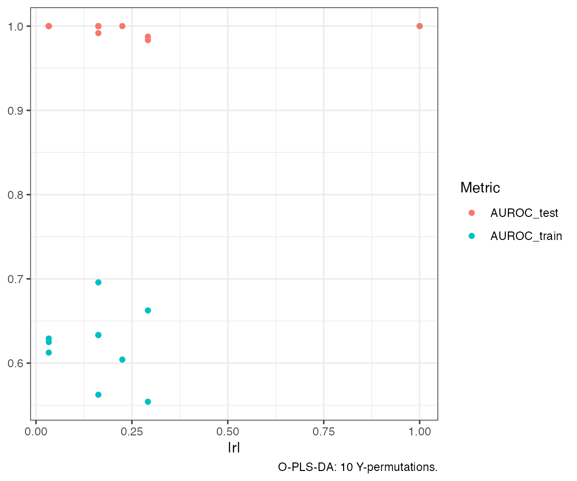

Model Diagnostics

Use dmodx() to assess outliers based on distance to the model in X-space (DModX):

distanceX<-dmodx(mod =opls.model, plot=TRUE)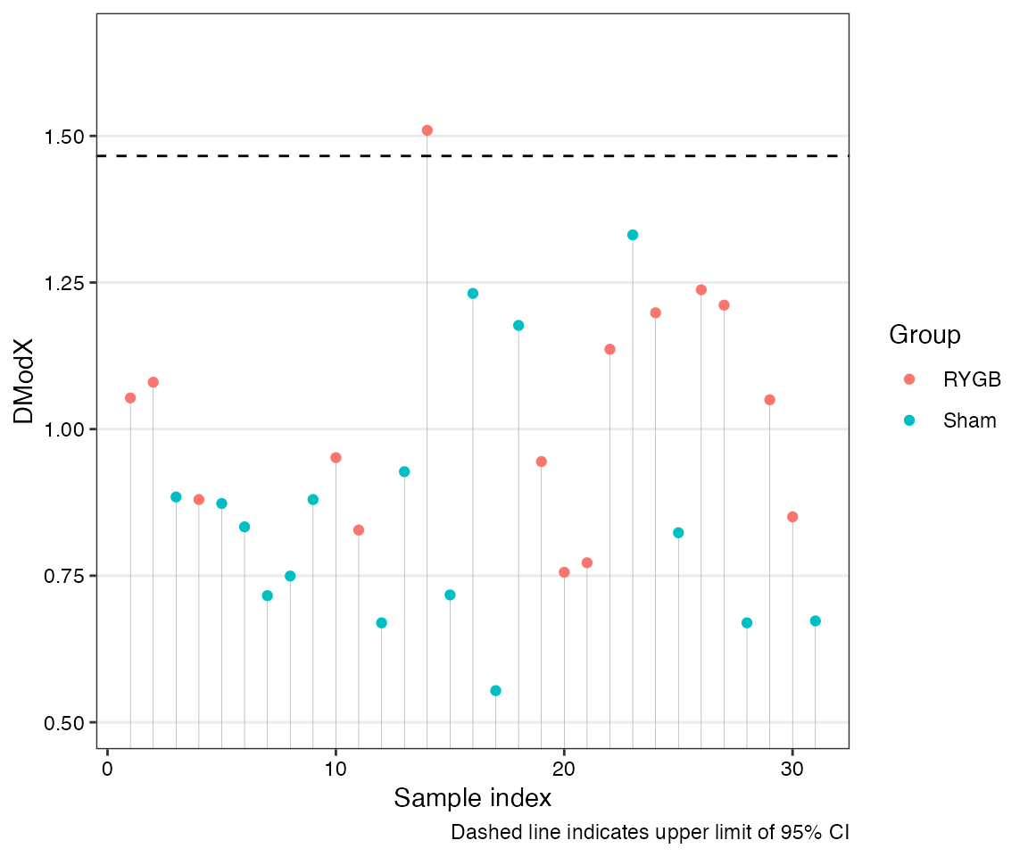

Samples above the 95% confidence line warrant inspection.

Visualising O-PLS Scores and Loadings

Scores plots summarise group separation. plotscores() includes options for aesthetics and cross-validated scores:

# Plot OPLS scores
plotscores(obj=opls.model, an=list(
  Surgery=an$Class[idx],          # colouring according to surgery type
  Timepoint=an$Timepoint[idx]),   # line type according to time point
  title='OPLS - Scores plot',     # plot title
  cv.scores = TRUE)               # visualise cross-validated scores

The predictive component is along the x-axis. The orthogonal component (y-axis) is unrelated to the outcome and often reflects technical variation (e.g., batch or normalisation effects).

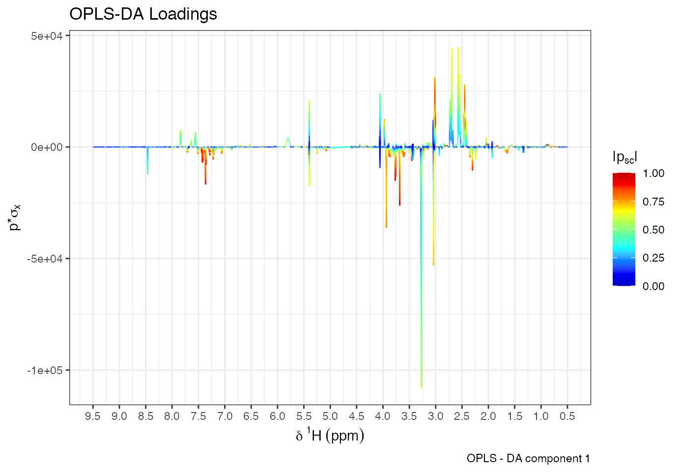
Variable Importance: Loadings & Spectral Mapping

Use plotload() to visualise variable contributions:

plotload(opls.model, type="Statistical reconstruction", title = 'Stat. Reconstructed Loadings', shift = c(0.5, 9.5))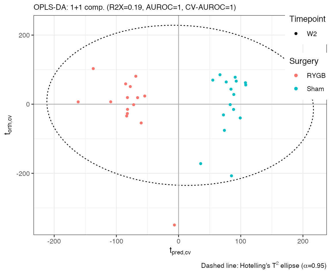

Backscaled loadings map effects onto spectral units:

plotload(opls.model, type = "backscaled", title = "Backscaled Loadings", shift = c(0.5, 9.5))

Overlay backscaled loadings with group spectra using specload():

specload(mod=opls.model, shift=c(7.3,7.45), an=list(
  facet=an$Class[idx]), 
  type='backscaled', 
  alp = 0.5, 
  title = 'Overlayed Spectra with Backscaled Loadings')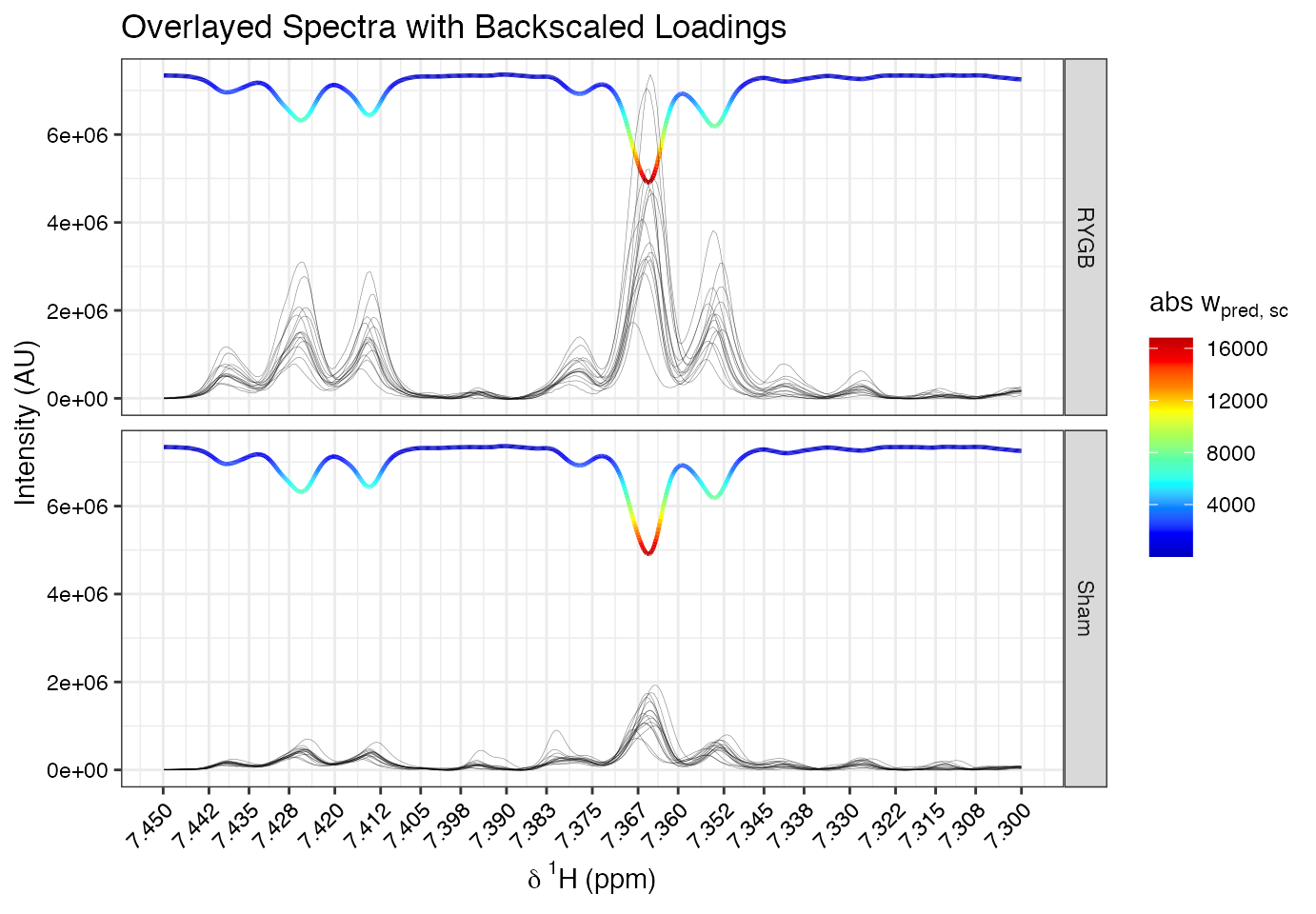

This reveals that signals at ~7.365 and ~7.425 ppm are stronger in the RYGB group, indicating their role in group separation.

Metabolite Identification

Once important variables are identified through supervised modeling (e.g., O-PLS), the next step is to group co-varying signals that may originate from the same metabolite.

Statistical Total Correlation Spectroscopy (STOCSY)

Metabolites often give rise to multiple resonances in NMR spectra. STOCSY is a correlation-based method that helps identify structurally related peaks, aiding compound annotation.

# define driver peak (the ppm variable where all other spectral variables will be correlated to)
driver1<-7.834
# perform stocsy
stocsy_model<-stocsy(Xn, ppm, driver1) 
# zoom-in different plot regions
plotStocsy(stocsy_model, shift=c(7,8))
plotStocsy(stocsy_model, shift=c(3.9, 4))

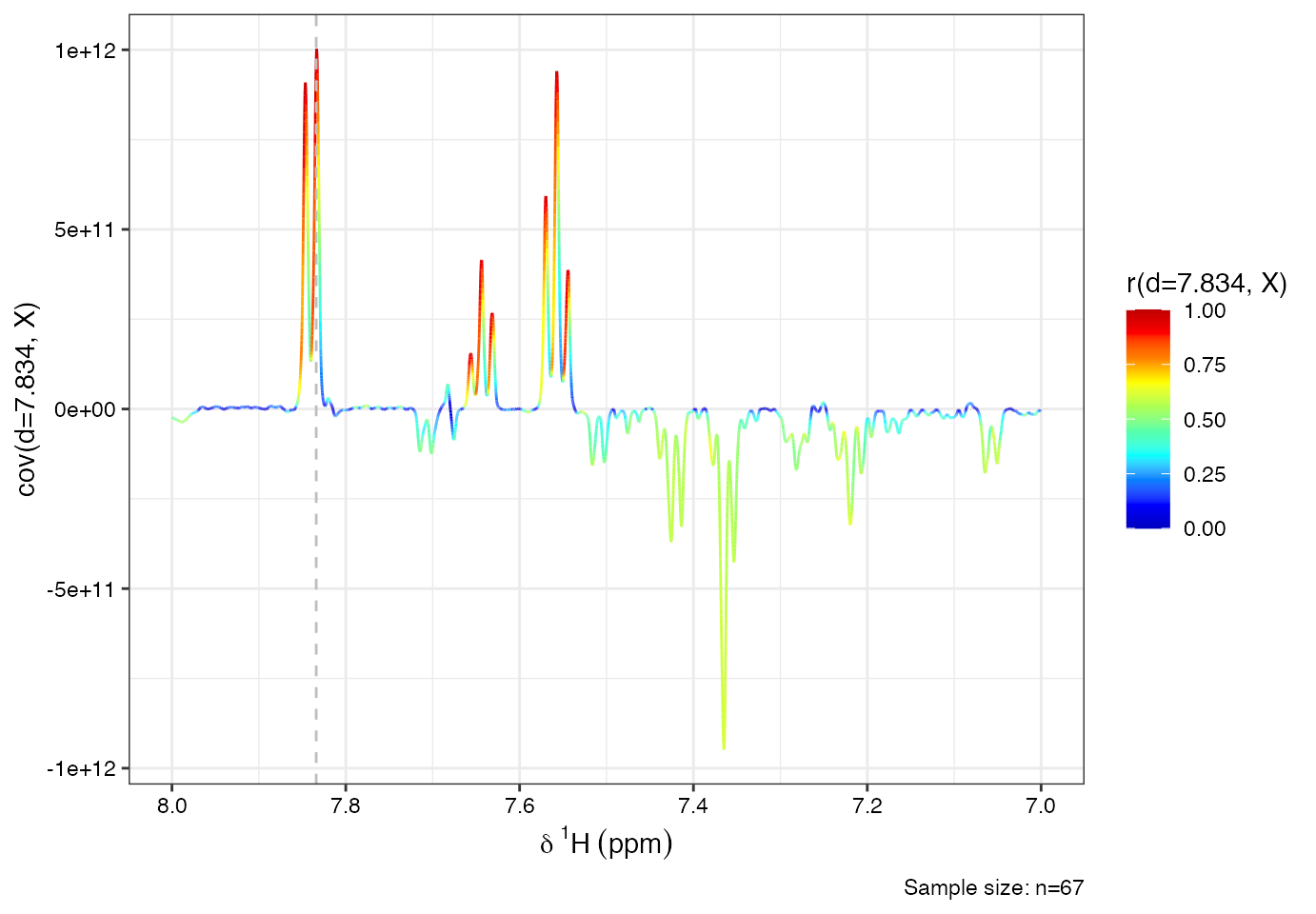
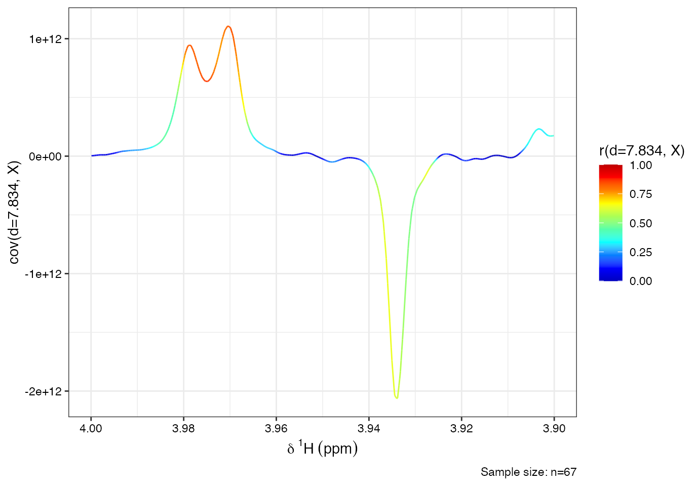From the STOCSY plot, you may observe multiple correlated peaks:

Multiplet @ 7.56 ppm
Multiplet @ 7.65 ppm
Doublet @ 7.84 ppm
Doublet @ 3.97 ppm These co-varying signals suggest they originate from the same compound.

Subset-Optimisation by Reference Matching (STORM)

# define driver peak (the ppm variable where all other spectral variables will be correlated to)
poi<-7.874
sig = 0.02
subset_idc <- storm(Xn, ppm, idx.refSpec = 2, shift=c(poi-sig, poi+sig), b=10)

storm_sets = rep('not_matched', nrow(Xn))
storm_sets[subset_idc] = 'matched'
table(storm_sets)
#> storm_sets
#>     matched not_matched 
#>           7          60

specOverlay(Xn, ppm, shift = c(poi-sig, poi+sig), an=list(type=storm_sets))

# run stocsy or spike-in's with respective storm spectra/samples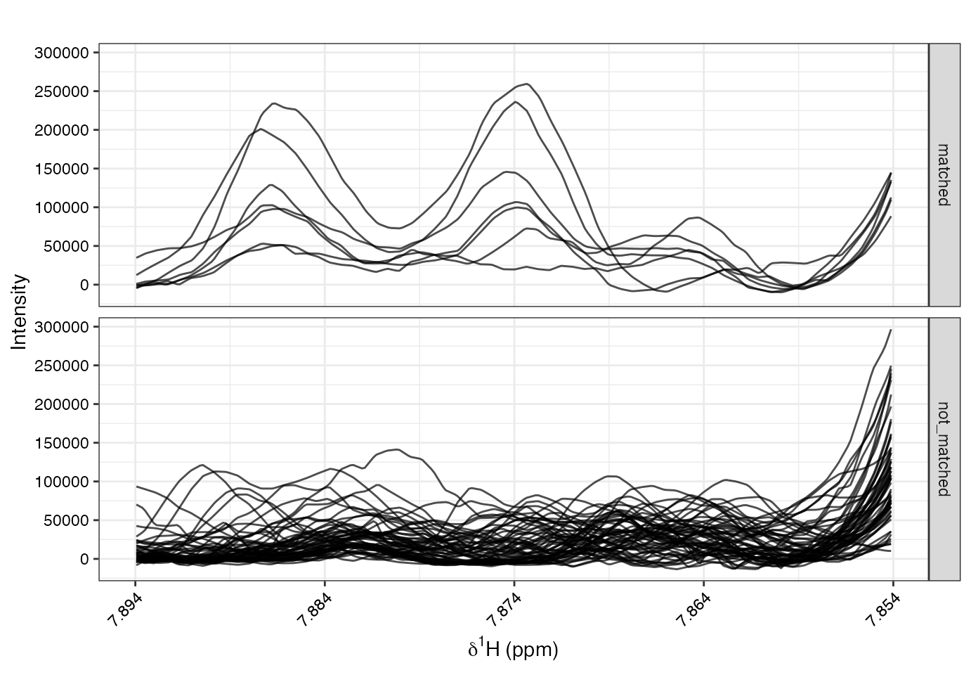

Spectral Database Query

Identified peak patterns can be queried against spectral reference databases to propose metabolite identities.

To query HMDB:

Go to www.hmdb.ca
Use the NMR search tool
Enter the chemical shifts (e.g., 7.84, 7.65, 7.56, 3.97)
Set a tolerance (e.g., ±0.01 ppm)

This provides a shortlist of candidate metabolites based on spectral matches.

cat("> **Note:** This method provides only a preliminary compound suggestion. Further NMR validation is recommended.\n\n")
#> > **Note:** This method provides only a preliminary compound suggestion. Further NMR validation is recommended.

Summary

This vignette introduced a chemometric workflow for NMR-based metabolic phenotyping using the metabom8 package. Key steps included: - Dimensionality reduction with PCA to visualise global trends - Supervised modeling with O-PLS to isolate treatment-associated variation - Visualisation of scores and loadings to interpret variable contributions - Identification of outliers and orthogonal structure via diagnostics - Use of STOCSY to highlight structurally linked signals - Querying public NMR databases to support metabolite identification

Together, these tools streamline the exploration, interpretation, and annotation of complex spectral datasets.

Citation

To cite the metabom8 package in publications, use:

To cite metabom8, please use:

Kimhofer T (2025). metabom8: A High-Performance R Package for Metabolomics Modeling and Analysis (R package version 1.2.0). doi:10.5281/zenodo.16794445.

A BibTeX entry for LaTeX users is

@Manual{, title = {metabom8: A High-Performance R Package for Metabolomics Modeling and Analysis}, author = {Torben Kimhofer}, year = {2025}, note = {R package version 1.2.0}, doi = {10.5281/zenodo.16794445}, url = {https://doi.org/10.5281/zenodo.16794445}, }

Session Info

#> R version 4.5.1 (2025-06-13)
#> Platform: aarch64-apple-darwin20
#> Running under: macOS Sequoia 15.5
#> 
#> Matrix products: default
#> BLAS:   /Library/Frameworks/R.framework/Versions/4.5-arm64/Resources/lib/libRblas.0.dylib 
#> LAPACK: /Library/Frameworks/R.framework/Versions/4.5-arm64/Resources/lib/libRlapack.dylib;  LAPACK version 3.12.1
#> 
#> locale:
#> [1] C/UTF-8/C/C/C/C
#> 
#> time zone: Europe/Berlin
#> tzcode source: internal
#> 
#> attached base packages:
#> [1] stats     graphics  grDevices utils     datasets  methods   base     
#> 
#> other attached packages:
#> [1] metabom8_0.99.0  nmrdata_0.1.0    BiocStyle_2.36.0
#> 
#> loaded via a namespace (and not attached):
#>  [1] gtable_0.3.6        ellipse_0.5.0       xfun_0.52          
#>  [4] bslib_0.9.0         ggplot2_3.5.2       htmlwidgets_1.6.4  
#>  [7] ggrepel_0.9.6       Biobase_2.68.0      vctrs_0.6.5        
#> [10] tools_4.5.1         crosstalk_1.2.1     generics_0.1.4     
#> [13] parallel_4.5.1      tibble_3.3.0        pkgconfig_2.0.3    
#> [16] data.table_1.17.8   RColorBrewer_1.1-3  desc_1.4.3         
#> [19] lifecycle_1.0.4     compiler_4.5.1      farver_2.1.2       
#> [22] stringr_1.5.1       ptw_1.9-16          textshaping_1.0.1  
#> [25] RcppDE_0.1.8        htmltools_0.5.8.1   sass_0.4.10        
#> [28] yaml_2.3.10         lazyeval_0.2.2      plotly_4.11.0      
#> [31] pillar_1.11.0       pkgdown_2.1.3       jquerylib_0.1.4    
#> [34] tidyr_1.3.1         MASS_7.3-65         cachem_1.1.0       
#> [37] abind_1.4-8         pcaMethods_2.0.0    tidyselect_1.2.1   
#> [40] digest_0.6.37       stringi_1.8.7       dplyr_1.1.4        
#> [43] reshape2_1.4.4      purrr_1.1.0         bookdown_0.43      
#> [46] labeling_0.4.3      fastmap_1.2.0       grid_4.5.1         
#> [49] cli_3.6.5           magrittr_2.0.3      withr_3.0.2        
#> [52] scales_1.4.0        rmarkdown_2.29      httr_1.4.7         
#> [55] signal_1.8-1        ragg_1.4.0          evaluate_1.0.4     
#> [58] knitr_1.50          viridisLite_0.4.2   rlang_1.1.6        
#> [61] Rcpp_1.1.0          glue_1.8.0          BiocManager_1.30.26
#> [64] BiocGenerics_0.54.0 pROC_1.19.0.1       jsonlite_2.0.0     
#> [67] R6_2.6.1            plyr_1.8.9          systemfonts_1.2.3  
#> [70] fs_1.6.6            colorRamps_2.3.4

Torben Kimhofer

2025-08-11