Fit an Orthogonal Partial Least Squares (O-PLS) model

Fits a supervised Orthogonal Partial Least Squares (O-PLS) model using a NIPALS-based algorithm with optional cross-validation and automatic component selection.

Usage

opls(X, Y, scaling, validation_strategy)

Arguments

X: Numeric matrix of predictors (rows = samples, columns = variables).
Y: Numeric matrix or factor vector of responses.
scaling: A scaling strategy object (e.g., uv_scaling(center = TRUE)), specifying model-internal centering and/or scaling applied during fitting. This does not modify the original spectral matrix.
validation_strategy: A cross-validation strategy object defining how resampling is performed (e.g., k-fold, Monte Carlo).

Value

An object of class m8_model containing the fitted O-PLS model, cross-validation results, and performance statistics.

Details

O-PLS decomposes the predictor matrix into:

One predictive component capturing variation correlated with Y
Orthogonal components capturing structured variation in X unrelated to Y

Predictive and orthogonal components are estimated sequentially. Cross-validated performance metrics (e.g., Q², R², classification AUC) are computed for each model configuration according to the supplied validation_strategy.

The model extracts a single predictive component and iteratively adds orthogonal components until the stopRule indicates overfitting or maxPCo is reached.

Scaling specified via scaling is applied internally during model fitting and does not alter the input matrix X. Spectral preprocessing (e.g., alignment or baseline correction) should be performed prior to model fitting.

The returned model object stores:

Predictive and orthogonal component models
Cross-validation results
Performance metrics (R², Q², AUC)
Model control parameters
Input data provenance metadata
Session information for reproducibility

Examples

data(covid)

cv <- balanced_mc(k=5, split=2/3)
scaling <- uv_scaling(center=TRUE)
model <-opls(X=covid$X, Y=covid$an$type, scaling, cv)
#> Performing discriminant analysis.
#> An O-PLS-DA model with 1 predictive and 1 orthogonal components was fitted.

show(model)
#> 
#> m8_model <opls>
#> ----------------------------------------
#> Dimensions  : 10 samples x 27819 variables
#> Mode        : classification 
#> Preprocess  : center | UV 
#> Components  : 2 (3 tested)
#> Validation  : BalancedMonteCarlo (k = 5) 
#> Stop rule   : cv_improvement_negligible 
#> ----------------------------------------
#> Use summary() for performance metrics.
#> 
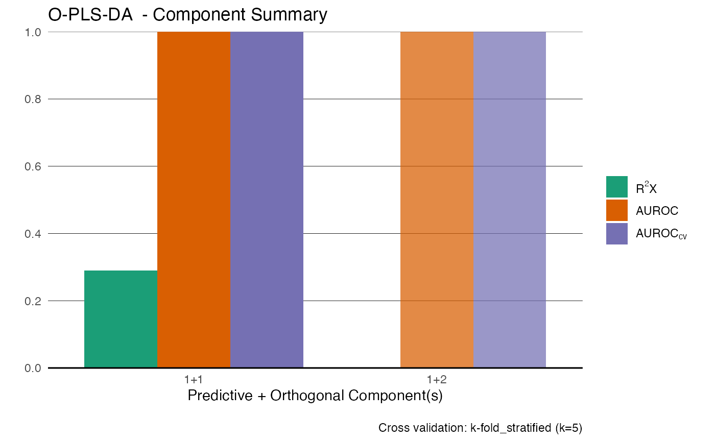
summary(model)
#> $perf
#>   comp_total comp_pred comp_orth AUCt AUCv       R2X selected        fit
#> 1          2         1         1    1    1 0.2860832     TRUE     fitted
#> 2          3         1         2    1    1        NA    FALSE not fitted
#>                 stop_reason stop_metric stop_delta
#> 1                      <NA>          NA         NA
#> 2 cv_improvement_negligible           1          0
#> 
#> $engine
#> [1] "opls"
#> 
#> $y_type
#> [1] "DA"
#> 

# scores
Tp <- scores(model)
To <- scores(model, orth=TRUE)

t2 <- hotellingsT2(cbind(Tp, To))
ell <-ellipse2d(t2)

plot(Tp, To, asp = 1,
  col = as.factor(covid$an$type),
  xlim = range(c(Tp, ell$x)),
  ylim = range(c(To, ell$y))
 )
lines(ell$x, ell$y, col = "grey", lty=2)


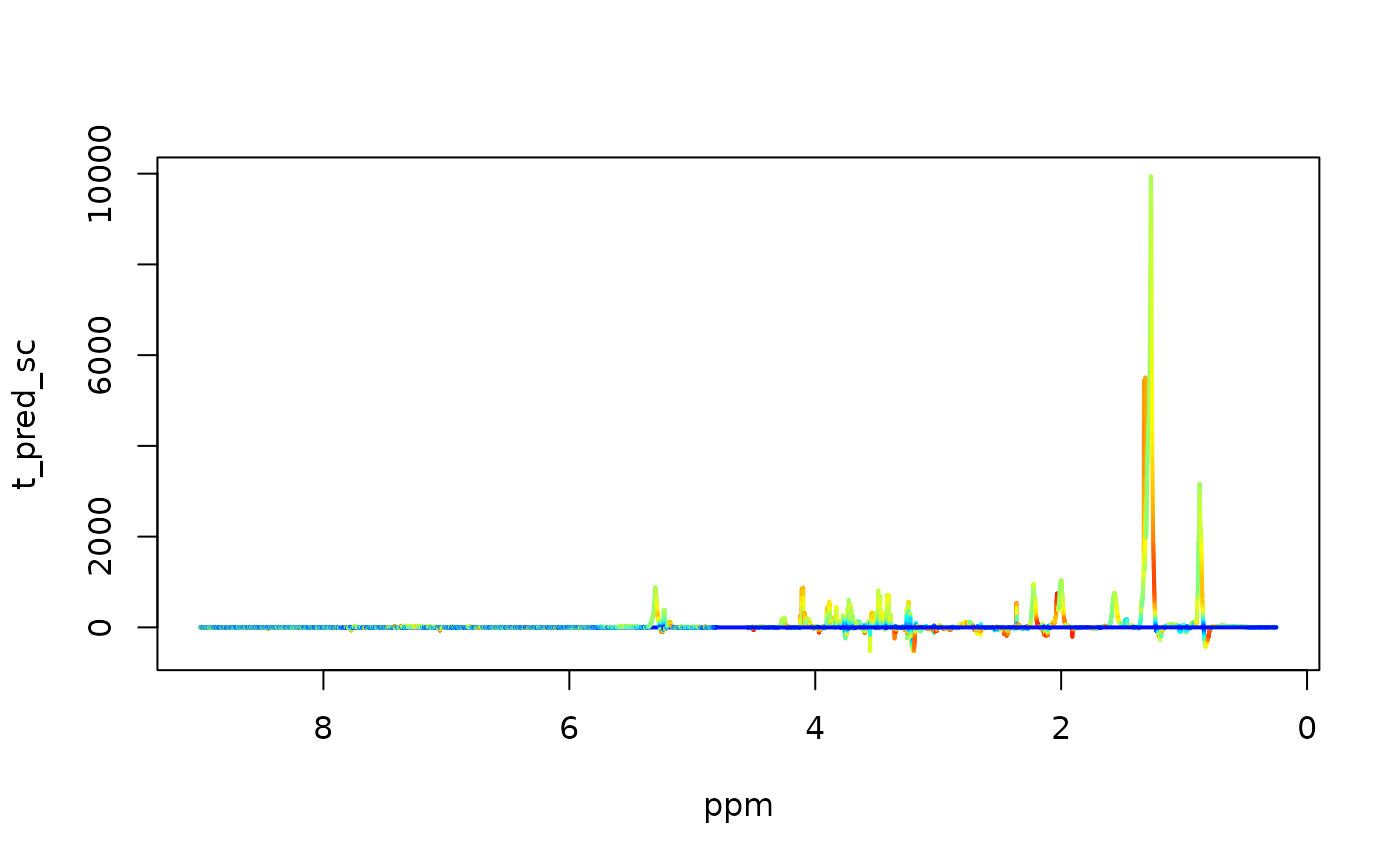
# loadings & vip's
Pp <- loadings(model)
Po <- loadings(model, orth=TRUE)
vips <- vip(model)

x=covid$ppm
y = Pp * apply(covid$X, 2, sd)

palette <-  colorRampPalette(c("blue", "cyan", "yellow", "red"))(100)
idx <- cut(vips, breaks = 100, labels = FALSE)
plot(x, y, type = "n", xlim = rev(range(x)), xlab='ppm', ylab='t_pred_sc')

for (i in seq_len(length(x) - 1)) {
  segments(x[i], y[i], x[i+1], y[i+1], col = palette[idx[i]], lwd = 2)
}