Plot PCA, PLS or OPLS Model Scores

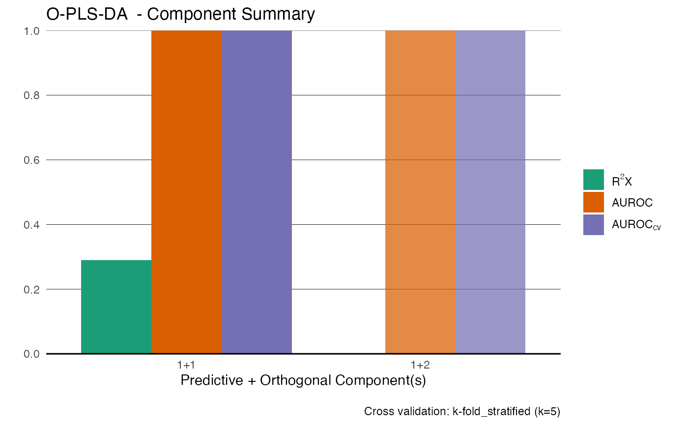
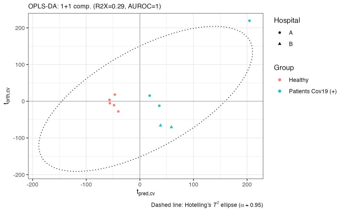
Generate score plots for PCA, PLS, or OPLS models with optional annotation, QC highlighting, and cross-validation scores.

Usage

plotscores(obj, pc, an, title = "", qc, legend = "in", cv = TRUE, ...)

Arguments

obj

A fitted model object of class PCA_metabom8, OPLS_metabom8, PLS_metabom8

pc

Numeric or character vector of length 2. Principal components or score components to plot. Defaults: c(1,2) for PCA/PLS, c("1", "o1") for OPLS.

an

Optional list of up to 3 elements specifying annotation: list(color, shape, label).

title

Optional character. Plot title.

qc

Optional integer vector of row indices indicating QC samples to highlight.

legend

Character. Legend position inside plot (default), or set to NA to suppress.

cv

Logical. If TRUE, cross-validated scores are shown when available (OPLS only).

...

Additional arguments passed to scale_colour_gradientn.

Value

A ggplot2 object.

References

Trygg J., Wold S. (2002) Orthogonal projections to latent structures (O-PLS). Journal of Chemometrics, 16(3):119–128. Hotelling H. (1931) The generalization of Student’s ratio. Annals of Mathematical Statistics, 2:360–378.

Examples

data("covid")
X <- covid$X
an <- covid$an

y = an$type
mod = opls(X, y)
#> Performing discriminant analysis.
#> Reducing k to 5 due to small group size (min n = 5).
#> An O-PLS-DA model with 1 predictive and 1 orthogonal components was fitted.

plotscores(mod, an=list(Group=y, Hospital=an$hospital))