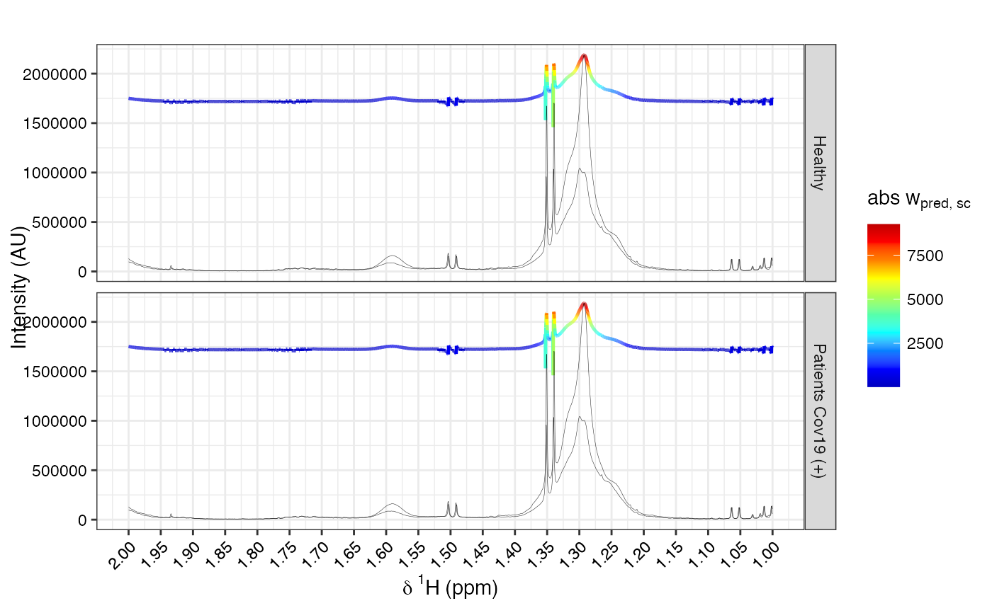
This function overlays loadings from a PCA or OPLS model on top of NMR spectra using ggplot2.
It supports two types of loadings visualization: statistical reconstruction or backscaling.
Usage
specload(
  mod,
  shift = c(0, 10),
  an,
  alp = 0.3,
  size = 0.5,
  pc = 1,
  type = "Backscaled",
  title = "",
  r_scale = FALSE
)
Arguments
- mod
A model object of class
PCA_metabom8orOPLS_metabom8.- shift
Numeric vector (length 2), chemical shift region to visualize (in ppm).
- an
List of up to three grouping variables (for facet, color, linetype). First must be defined.
- alp
Numeric (0–1). Alpha level for spectra.
- size
Numeric. Line width for plotted spectra.
- pc
Integer. Component to visualize (for OPLS, set to 1).
- type
Character. Either
"Statistical reconstruction"or"Backscaled"(case-insensitive).- title
Character. Plot title.
- r_scale
Logical. If
TRUE, correlation color scale is fixed to[0, 1]. Only used in statistical reconstruction.
Details
Statistical reconstruction: Correlates predictive scores with spectral variables.
Backscaled: Multiplies model loadings by feature SDs.
