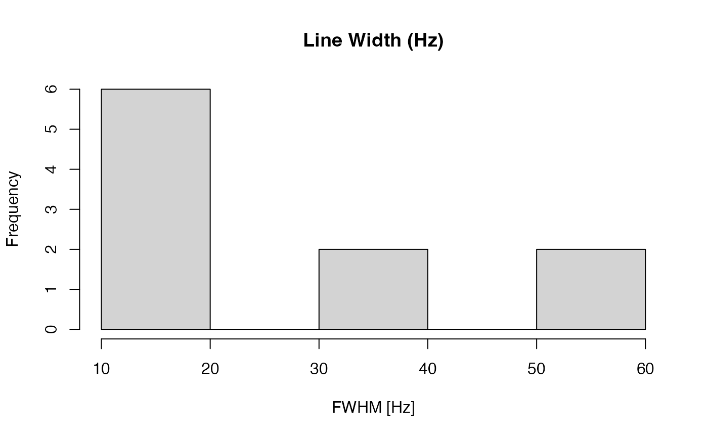
Estimates the full width at half maximum (FWHM; line width) of a singlet-like peak within a specified chemical-shift range for each spectrum.
Usage
lw(X, ppm = NULL, shift = c(-0.1, 0.1), sf)Arguments
- X
Numeric matrix (spectra in rows) or a named list as returned by
read1d/read1d_proccontainingX,ppm, andmeta.- ppm
Numeric vector of chemical shift values (ppm) corresponding to columns of
X. IfNULL,ppmis inferred in the following order:attr(X, "m8_axis")$ppm(if present),numeric
colnames(X)(if present).
- shift
Numeric vector of length 2. Chemical shift range containing the peak (e.g.,
c(-0.1, 0.1)for TSP).- sf
Spectrometer frequency in MHz. Either a single numeric (recycled across spectra) or a numeric vector of length
nrow(X)(one value per spectrum). IfXis a list input andsfis missing,sfis taken fromX$meta$a_SFO1when available. Ifsfis missing for a matrix input, the function attempts to useattr(X, "m8_meta")$a_SFO1when present.
Details
For each spectrum, the function:
extracts the region defined by
shift,finds the peak apex within that region,
computes the half-height level relative to the local baseline (minimum in the window),
estimates the left and right half-height crossing points by linear interpolation,
converts the width from ppm to Hz using
sf(MHz), i.e.Hz = ppm * sf.
If no valid half-height crossings can be found (e.g., very low SNR or truncated peak),
NA is returned for that spectrum.
Note
The ppm axis may be increasing or decreasing; FWHM is computed as an absolute width and is therefore independent of axis direction.
Examples
# Simulated NMR peaks with different linewidths
ppm <- seq(-0.2, 0.2, length.out = 1000)

# generate peaks with increasing width
sds <- seq(0.01, 0.03, length.out = 10)

X <- t(sapply(sds, function(s)
  dnorm(ppm, mean = 0, sd = s)
))

sf <- 600  # spectrometer frequency in MHz

fwhm_vals <- lw(X, ppm = ppm, shift = c(-0.1, 0.1), sf = sf)

plot(sds, fwhm_vals,
  xlab = "Gaussian sd",
  ylab = "Estimated FWHM (Hz)",
  pch = 16)